Australian hindcast skill#

This page contains plots showing the skill of quantities averaged over the Natural Resource Management (NRM) super-cluster regions (see NRM-regions). As for the generic skill results, plots are shown for CAFE-f6 and for the CanESM5 and EC-Earth3 CMIP6 DCPP submissions (where possible). Note that much of the following work was motivated by deliverables for the Australian Climate Services (ACS) project.

[1]:

import warnings

warnings.filterwarnings("ignore")

import geopandas

import xarray as xr

import matplotlib.pyplot as plt

from src import utils, plot

from notebook_helper import plot_metrics, plot_metric_maps, plot_hindcasts

[2]:

%load_ext autoreload
%autoreload 2
%load_ext lab_black

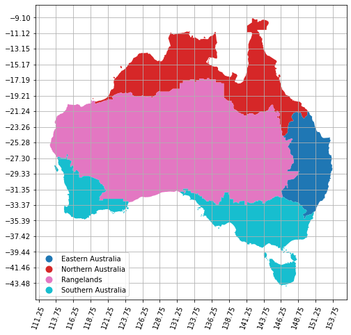
Focus regions#

In the following we’ll show some skill results for the following NRM super clusters and for the average over all of Australia. Note, the grid below shows the native CAFE atmospheric model grid.

[3]:

fig, ax = plt.subplots(1, 1, figsize=(8, 8))
df = geopandas.read_file("../data/raw/NRM_super_clusters/NRM_super_clusters.shp")
_ = df.plot("label", ax=ax, legend=True, legend_kwds={"loc": "lower left"})

data = xr.open_zarr(
    "../data/processed/CAFE_hist.annual.days_over_0.ehf_severity_Aus.zarr"
)
ax.set_xticks(data.lon.values, labels=data.lon.values, rotation=70)
ax.set_yticks(data.lat.values)
ax.grid()

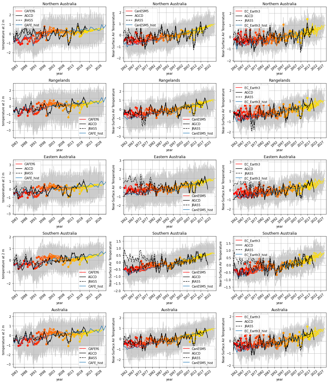
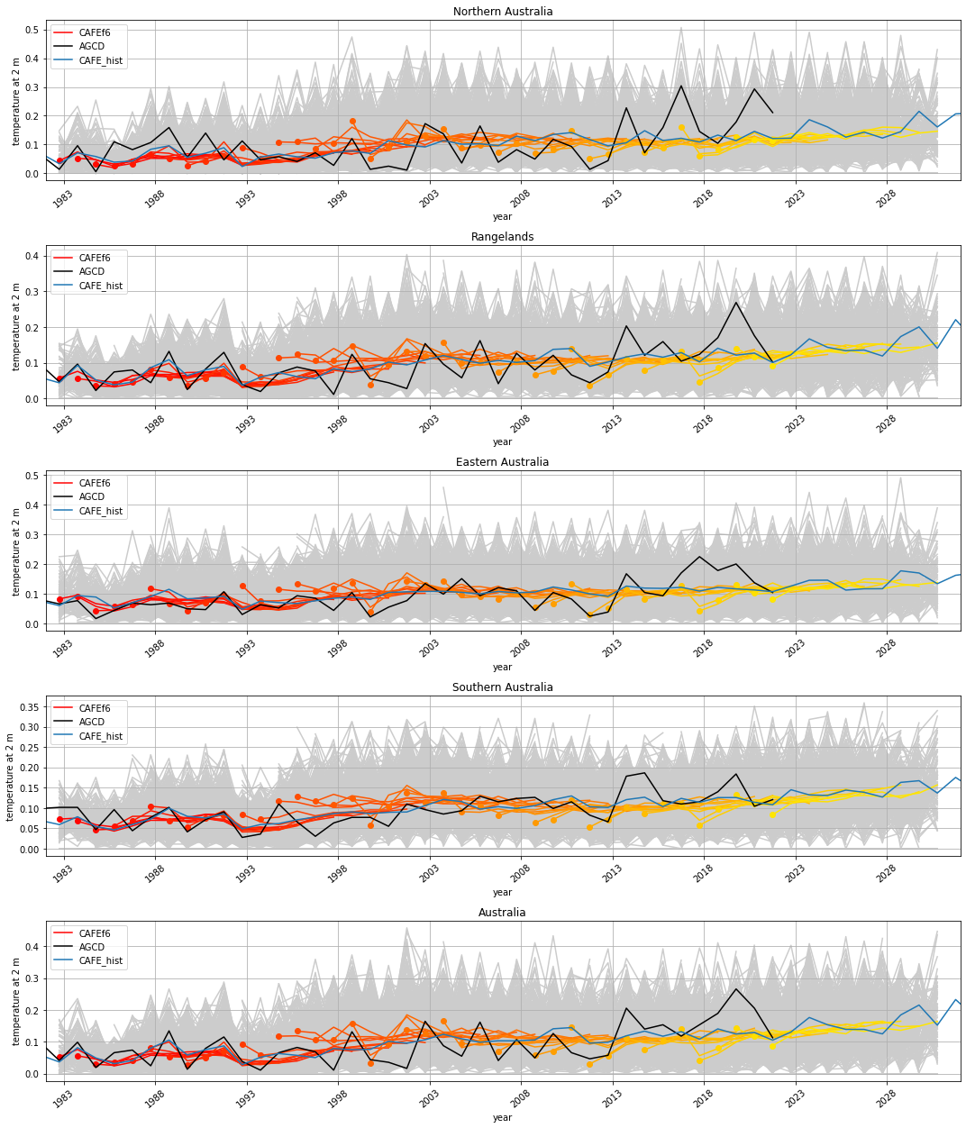
../_images/notebooks_assessment_Aus_4_0.png

Near-surface (2m) temperature relative to AGCD#

[4]:

plot_hindcasts(
    ["CAFEf6", "CanESM5", "EC_Earth3"],
    ["CAFE_hist", "CanESM5_hist", "EC_Earth3_hist"],
    ["AGCD", "JRA55"],
    "annual",
    "t_ref",
    "Aus_NRM",
)

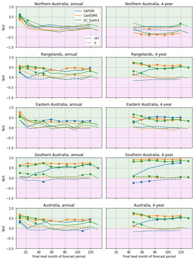
../_images/notebooks_assessment_Aus_6_0.png

Anomaly correlation coefficient (Pearson)#

[5]:

_ = plot_metrics(
    ["CAFEf6", "CanESM5", "EC_Earth3"],
    "AGCD",
    ["annual", "4-year"],
    "t_ref",
    ["rXY", "ri"],
    "Aus_NRM",
)

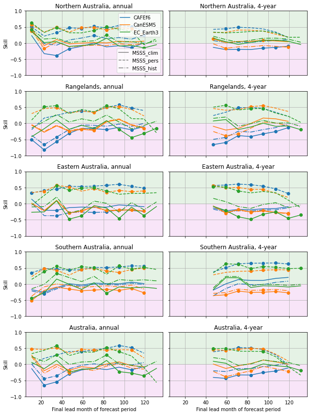
../_images/notebooks_assessment_Aus_8_0.png

Mean squared skill score#

[6]:

_ = plot_metrics(
    ["CAFEf6", "CanESM5", "EC_Earth3"],
    "AGCD",
    ["annual", "4-year"],
    "t_ref",
    ["MSSS_clim", "MSSS_pers", "MSSS_hist"],
    "Aus_NRM",
)

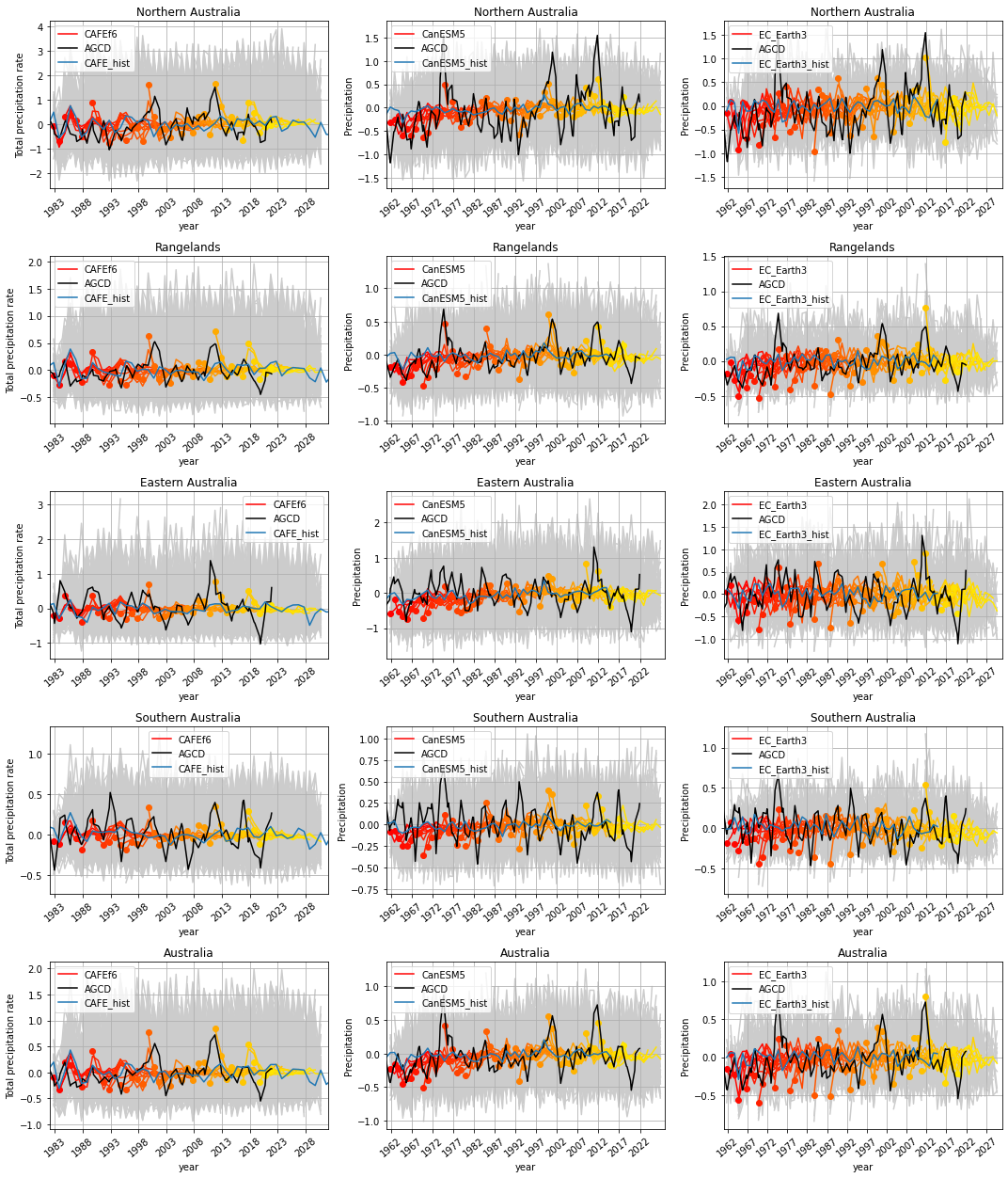
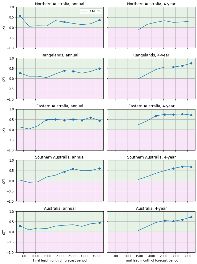
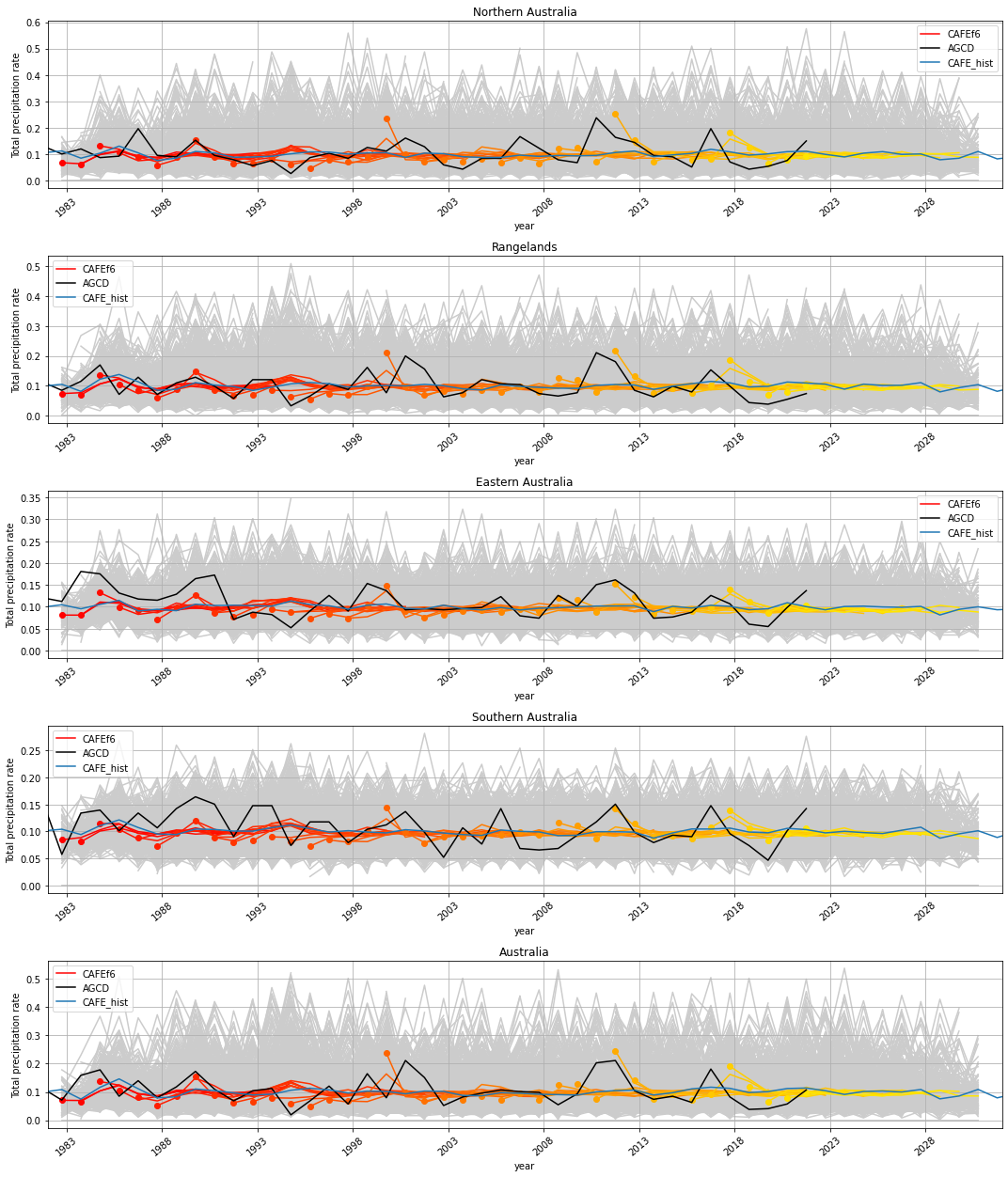
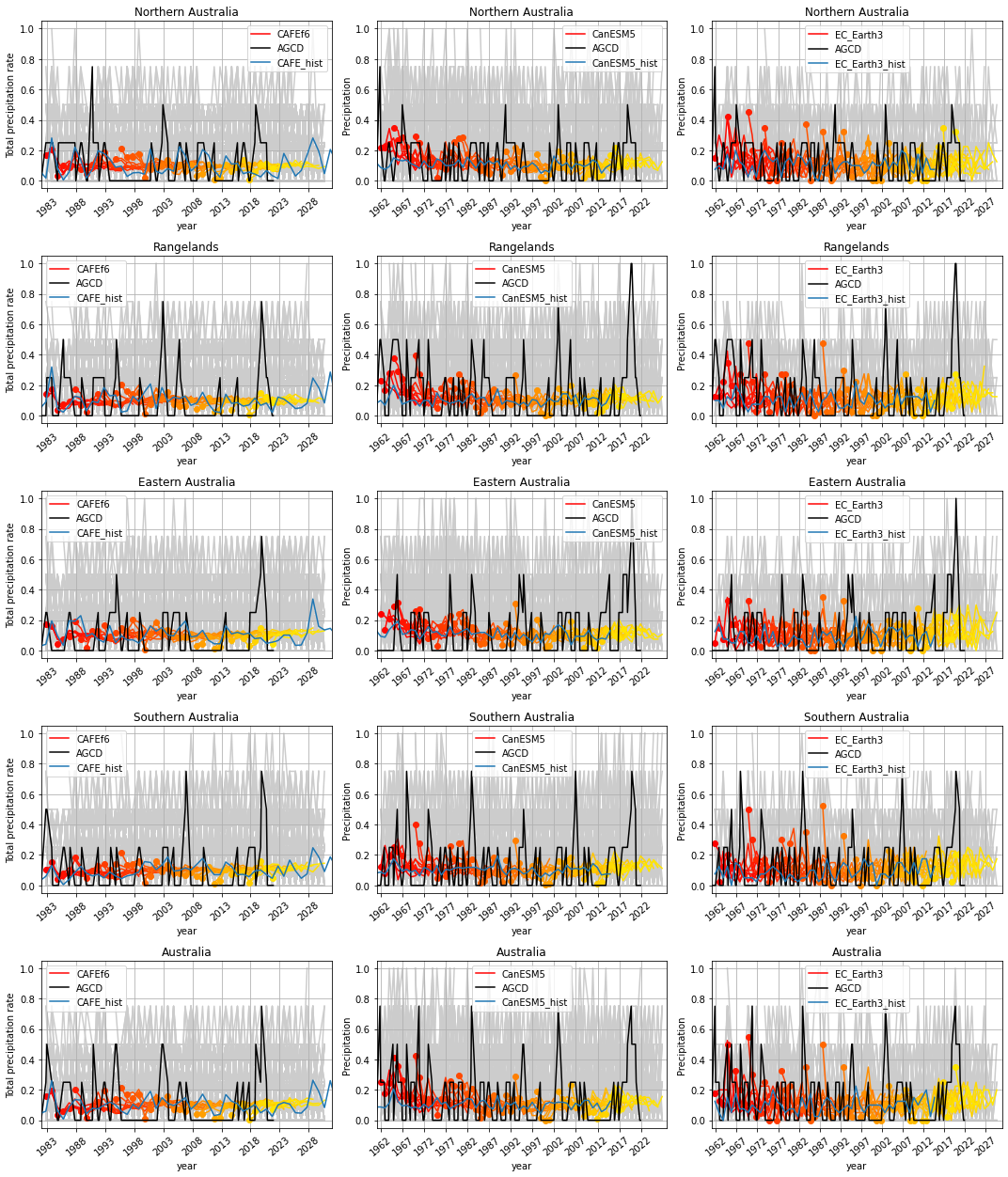
../_images/notebooks_assessment_Aus_10_0.png

Precipitation relative to AGCD#

[7]:

plot_hindcasts(
    ["CAFEf6", "CanESM5", "EC_Earth3"],
    ["CAFE_hist", "CanESM5_hist", "EC_Earth3_hist"],
    ["AGCD"],
    "annual",
    "precip",
    "Aus_NRM",
)

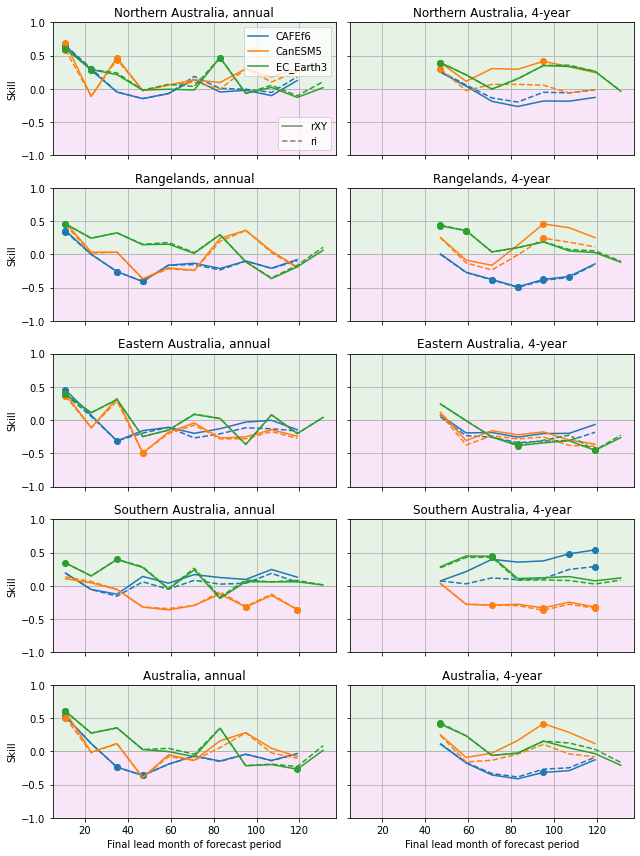
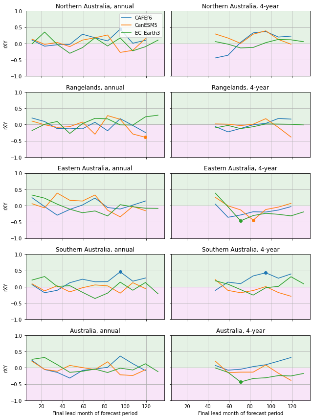
../_images/notebooks_assessment_Aus_12_0.png

Anomaly correlation coefficient (Pearson)#

[8]:

_ = plot_metrics(
    ["CAFEf6", "CanESM5", "EC_Earth3"],
    "AGCD",
    ["annual", "4-year"],
    "precip",
    ["rXY", "ri"],
    "Aus_NRM",
)

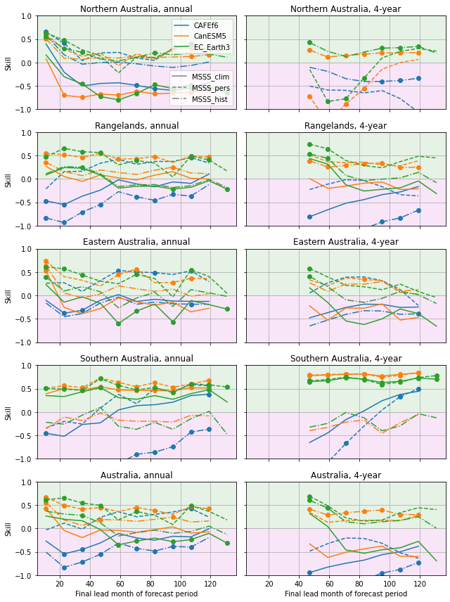
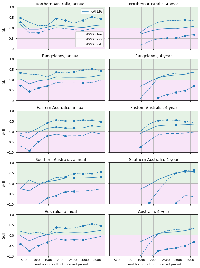
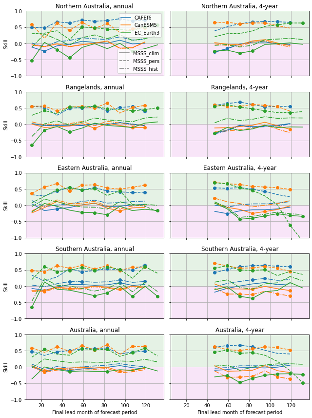
../_images/notebooks_assessment_Aus_14_0.png

Mean squared skill score#

[9]:

_ = plot_metrics(
    ["CAFEf6", "CanESM5", "EC_Earth3"],
    "AGCD",
    ["annual", "4-year"],
    "precip",
    ["MSSS_clim", "MSSS_pers", "MSSS_hist"],
    "Aus_NRM",
)

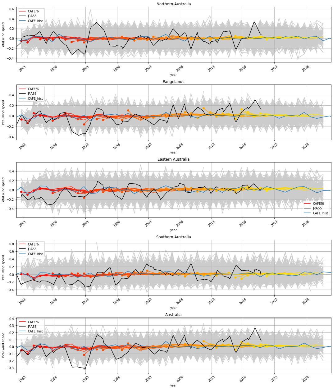
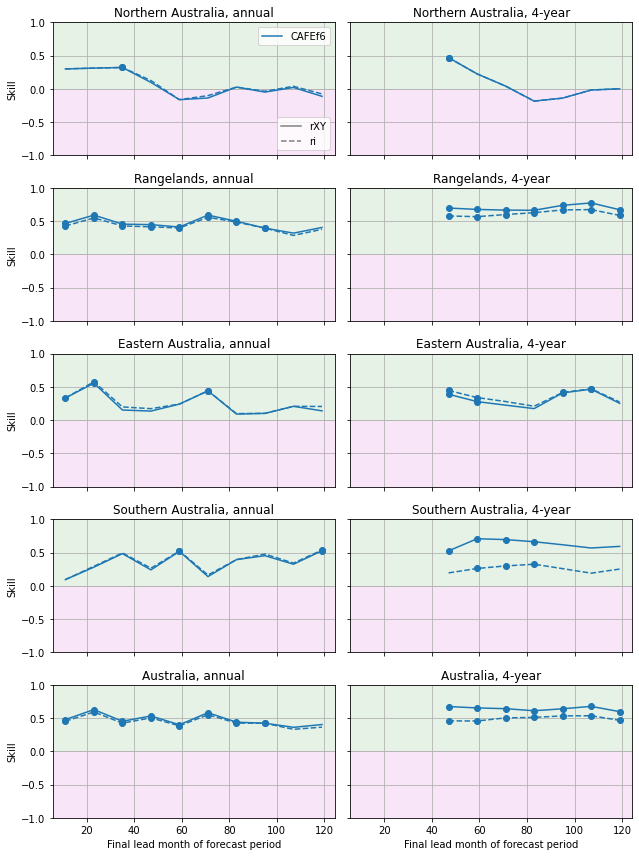
../_images/notebooks_assessment_Aus_16_0.png

Near-surface (10m) wind relative to JRA55#

[10]:

plot_hindcasts(["CAFEf6"], ["CAFE_hist"], ["JRA55"], "annual", "V_tot", "Aus_NRM")

../_images/notebooks_assessment_Aus_18_0.png

Anomaly correlation coefficient (Pearson)#

[11]:

_ = plot_metrics(
    ["CAFEf6"], "JRA55", ["annual", "4-year"], "V_tot", ["rXY", "ri"], "Aus_NRM"
)

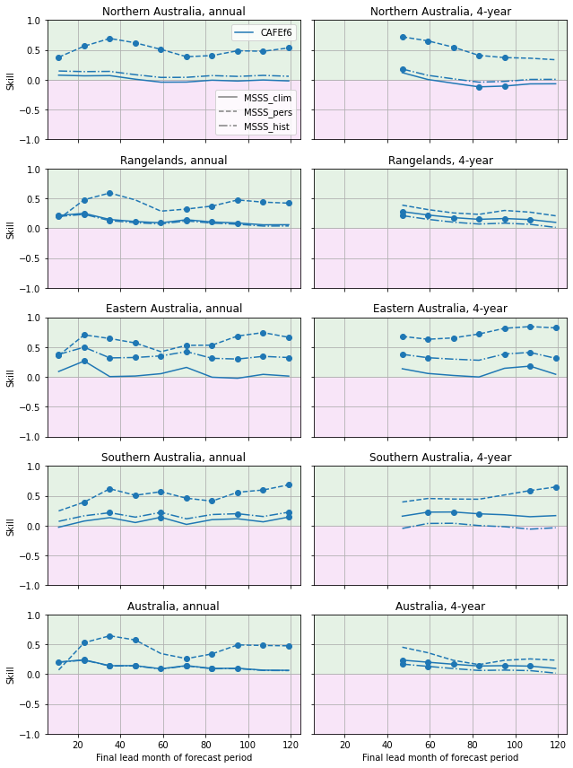
../_images/notebooks_assessment_Aus_20_0.png

Mean squared skill score#

[12]:

_ = plot_metrics(
    ["CAFEf6"],
    "JRA55",
    ["annual", "4-year"],
    "V_tot",
    ["MSSS_clim", "MSSS_pers", "MSSS_hist"],
    "Aus_NRM",
)

../_images/notebooks_assessment_Aus_22_0.png

Extreme 2m temperature relative to AGCD#

Here we assess the proportion of days in forecast period with maximum temperature over 90th percentile percentile. Percentile thresholds for each day-of-year are determined for each dataset from its own climatology over the period 1991-2020. In the case of hindcast data, percentile thresholds are determined for each lead time independently. All instances of Feb 29th are removed for all datasets to simplify processing.

[13]:

plot_hindcasts(
    ["CAFEf6"],
    ["CAFE_hist"],
    ["AGCD"],
    "annual",
    "t_ref_max",
    "Aus_NRM",
    "days_over_p90",
)

../_images/notebooks_assessment_Aus_24_0.png

Anomaly correlation coefficient (Spearman)#

[14]:

_ = plot_metrics(
    ["CAFEf6"],
    "AGCD",
    ["annual", "4-year"],
    "t_ref_max",
    ["rXY"],
    "Aus_NRM",
    "days_over_p90",
)

../_images/notebooks_assessment_Aus_26_0.png

Mean squared skill score#

[15]:

_ = plot_metrics(
    ["CAFEf6"],
    "AGCD",
    ["annual", "4-year"],
    "t_ref_max",
    ["MSSS_clim", "MSSS_pers", "MSSS_hist"],
    "Aus_NRM",
    "days_over_p90",
)

../_images/notebooks_assessment_Aus_28_0.png

Extreme precipitation relative to AGCD#

Here we assess the proportion of days in forecast period with precipitation over 90th percentile percentile. Percentile thresholds for each day-of-year are determined for each dataset from its own climatology over the period 1991-2020. In the case of hindcast data, percentile thresholds are determined for each lead time independently. All instances of Feb 29th are removed for all datasets to simplify processing.

[16]:

plot_hindcasts(
    ["CAFEf6"],
    ["CAFE_hist"],
    ["AGCD"],
    "annual",
    "precip",
    "Aus_NRM",
    "days_over_p90",
)

../_images/notebooks_assessment_Aus_30_0.png

Anomaly correlation coefficient (Spearman)#

[17]:

_ = plot_metrics(
    ["CAFEf6"],
    "AGCD",
    ["annual", "4-year"],
    "precip",
    ["rXY"],
    "Aus_NRM",
    "days_over_p90",
)

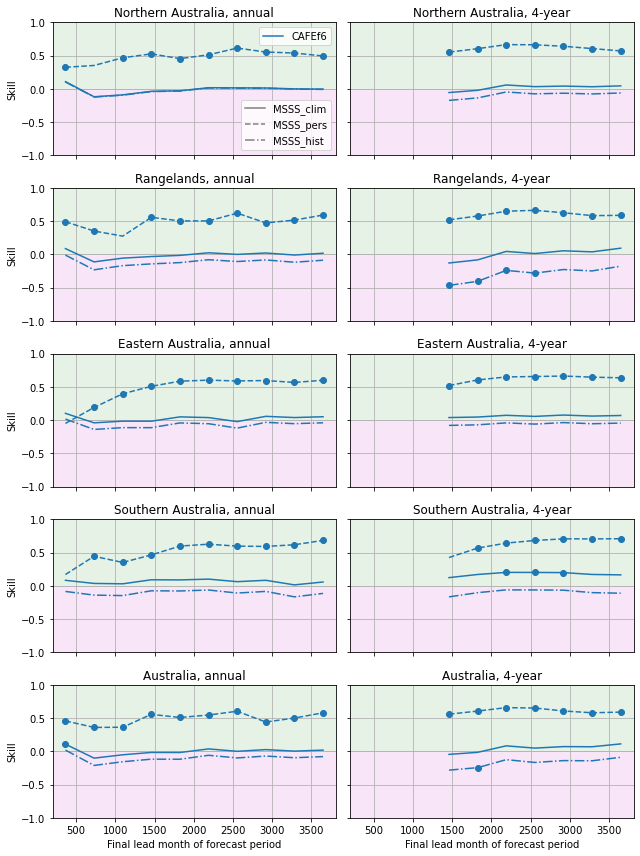
../_images/notebooks_assessment_Aus_32_0.png

Mean squared skill score#

[18]:

_ = plot_metrics(
    ["CAFEf6"],
    "AGCD",
    ["annual", "4-year"],
    "precip",
    ["MSSS_clim", "MSSS_pers", "MSSS_hist"],
    "Aus_NRM",
    "days_over_p90",
)

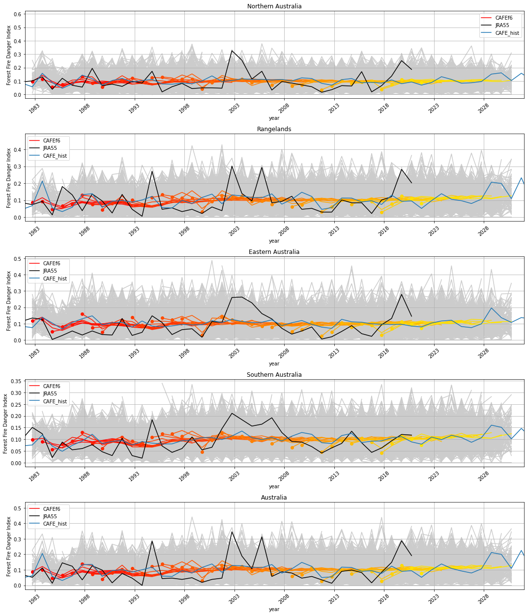
../_images/notebooks_assessment_Aus_34_0.png

Extreme Forest Fire Danger Index relative to JRA55#

Here we assess the proportion of days in forecast period with FFDI over 90th percentile percentile. Percentile thresholds for each day-of-year are determined for each dataset from its own climatology over the period 1991-2020. In the case of hindcast data, percentile thresholds are determined for each lead time independently. All instances of Feb 29th are removed for all datasets to simplify processing.

Note that FFDI is calculated in a non-standard way here due to data availability (see Richardson et al and Squire et al 2021):

At the moment, the drought factor is estimated as the 20-day accumulated rainfall normalised to lie between 0 and 10, with larger values indicating less precipitation. This tends to underpredict the number of very low FFDI days, but produces similar extreme values. The normalisation is carried out over all initial dates, lead times and ensemble members in the training period. This approach ensures that all days-of-year are included in the normalisation, however it does not account for lead-time dependent bias in precipitation.
Daily mean relative humidity at 1000 hPa is used rather than daily max relative humidity at 2 m
Daily mean wind speed at 10 m is used rather than daily max wind speed

[19]:

plot_hindcasts(
    ["CAFEf6"],
    ["CAFE_hist"],
    ["JRA55"],
    "annual",
    "ffdi",
    "Aus_NRM",
    "days_over_p90",
)

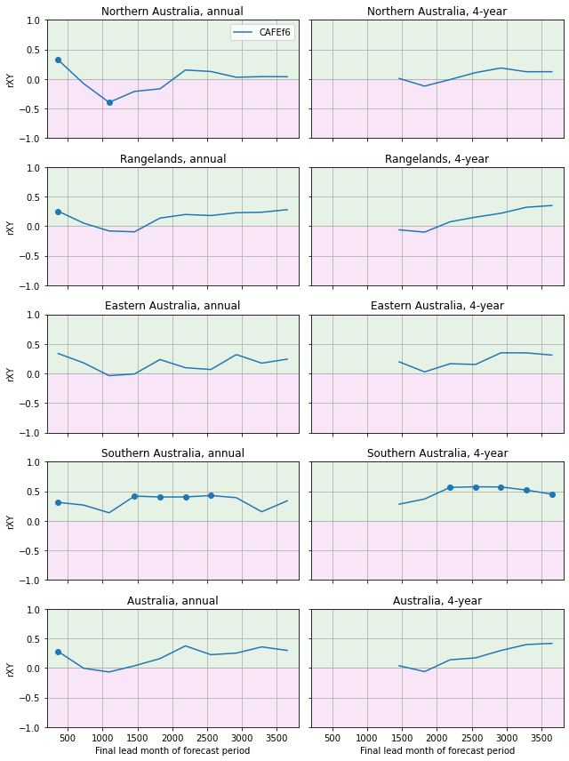
../_images/notebooks_assessment_Aus_36_0.png

Anomaly correlation coefficient (Spearman)#

[20]:

_ = plot_metrics(
    ["CAFEf6"],
    "JRA55",
    ["annual", "4-year"],
    "ffdi",
    ["rXY"],
    "Aus_NRM",
    "days_over_p90",
)

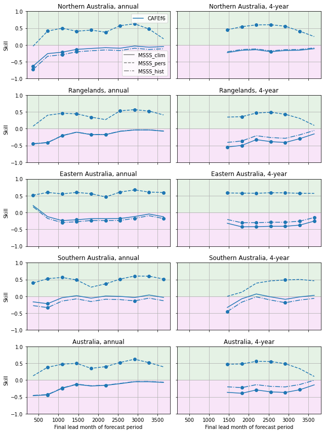
../_images/notebooks_assessment_Aus_38_0.png

Mean squared skill score#

[21]:

_ = plot_metrics(
    ["CAFEf6"],
    "JRA55",
    ["annual", "4-year"],
    "ffdi",
    ["MSSS_clim", "MSSS_pers", "MSSS_hist"],
    "Aus_NRM",
    "days_over_p90",
)

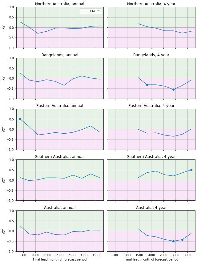
../_images/notebooks_assessment_Aus_40_0.png

Drought relative to AGCD#

Here a drought event is defined as when rainfall over a 3-month period is in the lowest decile (this is the Bureau of Meteorology definition, see Delage and Power 2020). We assess the proportion of 3-month periods in forecast period with precip within the first decile (equivalent to assessing the number of droughts in the forecast period). Note that the 3-month rainfall is not calculated in a rolling manner. Thus the max number of droughts in a year, for example, is 4. Percentile thresholds for each 3-month period are determined for each dataset from its own climatology over the period 1991-2020. In the case of hindcast data, percentile thresholds are determined for each lead time independently.

[22]:

plot_hindcasts(
    ["CAFEf6", "CanESM5", "EC_Earth3"],
    ["CAFE_hist", "CanESM5_hist", "EC_Earth3_hist"],
    ["AGCD"],
    "annual",
    "precip",
    "Aus_NRM",
    "3-months_under_p10",
)

../_images/notebooks_assessment_Aus_42_0.png

Anomaly correlation coefficient (Spearman)#

[23]:

_ = plot_metrics(
    ["CAFEf6", "CanESM5", "EC_Earth3"],
    "AGCD",
    ["annual", "4-year"],
    "precip",
    ["rXY"],
    "Aus_NRM",
    "3-months_under_p10",
)

../_images/notebooks_assessment_Aus_44_0.png

Mean squared skill score#

[24]:

_ = plot_metrics(
    ["CAFEf6", "CanESM5", "EC_Earth3"],
    "AGCD",
    ["annual", "4-year"],
    "precip",
    ["MSSS_clim", "MSSS_pers", "MSSS_hist"],
    "Aus_NRM",
    "3-months_under_p10",
)

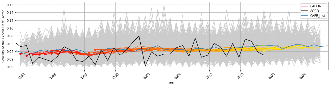
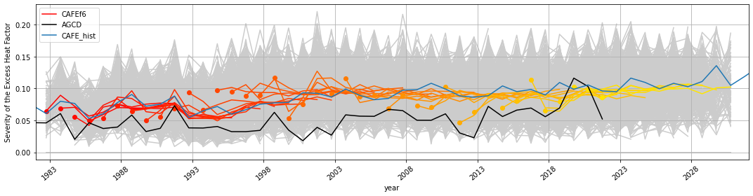
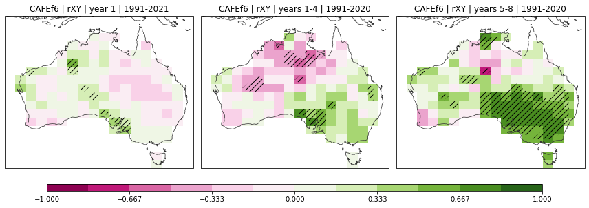
../_images/notebooks_assessment_Aus_46_0.png

Excess Heat Factor severity relative to AGCD#

Here, the excess heat factor (EHF) is calculated following Nairn and Fawcett 2015. To compute the EHF for the hindcasts, the daily temperature forecasts are first (additive) bias corrected over the verification period (1991-2020) relative to AGCD. The same is also true for the historical model data. The temperature and EHF percentiles used in the calculation of the hindcast/historical run EHF severity (T_95 and EHF_85) are calculated from AGCD over the Nairn and Fawcett periods: 1971-2000 and 1958-2011, respectively. Below we assess the proportion of days in forecast period with EHF severity over 0 (0-1: low-intensity heatwave; 1-3: severe but not extreme heatwave; > 3: extreme heatwave).

We present the following on the native CAFE grid since aggregation to larger regions presents issues with interpreting the magnitude of the EHF.

[25]:

plot_hindcasts(
    ["CAFEf6"], ["CAFE_hist"], ["AGCD"], "annual", "ehf_severity", "Aus", "days_over_0"
)

../_images/notebooks_assessment_Aus_48_0.png

Anomaly correlation coefficient (Spearman)#

[40]:

_ = plot_metric_maps(
    ["CAFEf6"],
    "AGCD",
    "ehf_severity",
    "rXY",
    "Aus",
    "days_over_0",
    figsize=(12, 4),
)

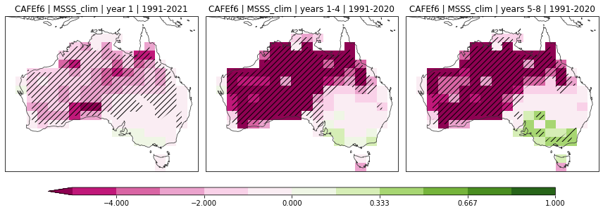
../_images/notebooks_assessment_Aus_50_0.png

Mean squared skill score relative to climatology#

[37]:

_ = plot_metric_maps(
    ["CAFEf6"],
    "AGCD",
    "ehf_severity",
    "MSSS_clim",
    "Aus",
    "days_over_0",
    vrange=(-5, 1),
    figsize=(12, 4),
)

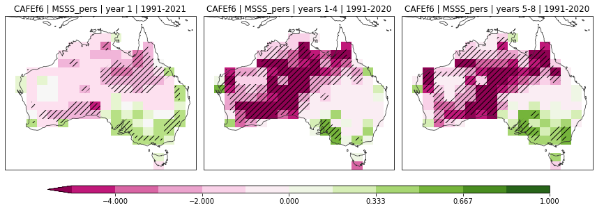
../_images/notebooks_assessment_Aus_52_0.png

Mean squared skill score relative to persistence#

[30]:

_ = plot_metric_maps(
    ["CAFEf6"],
    "AGCD",
    "ehf_severity",
    "MSSS_pers",
    "Aus",
    "days_over_0",
    vrange=(-5, 1),
    figsize=(12, 4),
)

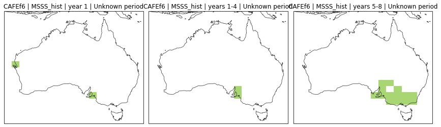
../_images/notebooks_assessment_Aus_54_0.png

Mean squared skill score relative to historical simulations#

[31]:

EHF_fig = plot_metric_maps(
    ["CAFEf6"],
    "AGCD",
    "ehf_severity",
    "MSSS_hist",
    "Aus",
    "days_over_0",
    vrange=(-5, 1),
    figsize=(12, 4),
)

../_images/notebooks_assessment_Aus_56_0.png

Where is the MSSS positive relative to climatology, persistence and historical simulations?#

Lighter green indicates both are positive; darker green indicates both are positive and significant

[32]:

EHF_fig = plot_metric_maps(
    ["CAFEf6"],
    "AGCD",
    "ehf_severity",
    ["MSSS_clim", "MSSS_pers", "MSSS_hist"],
    "Aus",
    "days_over_0",
    figsize=(12, 4),
)

../_images/notebooks_assessment_Aus_58_0.png

Annual hindcasts for the Adelaide grid box#

[33]:

loc = [138.75, -35.39]


def plot_loc(ax, loc):
    import cartopy.crs as ccrs

    ax.plot(
        loc[0], loc[1], "C3", marker="+", markersize=20, transform=ccrs.PlateCarree()
    )


for ax in EHF_fig.axes:
    plot_loc(ax, loc)

EHF_fig

[33]:

../_images/notebooks_assessment_Aus_60_0.png

[35]:

hcst = (
    xr.open_zarr("../data/processed/CAFEf6.annual.days_over_0.ehf_severity_Aus.zarr")
    .sel(lon=loc[0], lat=loc[1], method="nearest")
    .compute()
)
hist = (
    xr.open_zarr("../data/processed/CAFE_hist.annual.days_over_0.ehf_severity_Aus.zarr")
    .sel(lon=loc[0], lat=loc[1], method="nearest")
    .compute()
)
obsv = (
    xr.open_zarr("../data/processed/AGCD.annual.days_over_0.ehf_severity_Aus.zarr")
    .sel(lon=loc[0], lat=loc[1], method="nearest")
    .compute()
)

_ = plot.hindcasts({"CAFEf6": hcst}, {"AGCD": obsv}, {"CAFE_hist": hist})

../_images/notebooks_assessment_Aus_61_0.png