Generic hindcast skill#

This page contains plots showing the skill of commonly assessed variables and indices. Results are shown for CAFE-f6 and for the CanESM5 and EC-Earth3 CMIP6 DCPP submissions.

[1]:

import warnings

warnings.filterwarnings("ignore")

import cftime

import xarray as xr

import xskillscore as xs

import matplotlib.pyplot as plt

from src import utils, plot

from notebook_helper import plot_metrics, plot_metric_maps, plot_hindcasts

[2]:

%load_ext autoreload
%autoreload 2
%load_ext lab_black

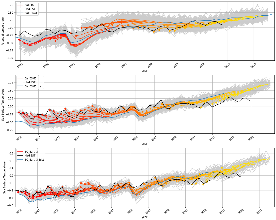
Sea surface temperature relative to HadISST#

Global average (60°S - 60°N) hindcast timeseries#

[3]:

plot_hindcasts(
    ["CAFEf6", "CanESM5", "EC_Earth3"],
    ["CAFE_hist", "CanESM5_hist", "EC_Earth3_hist"],
    ["HadISST"],
    "annual",
    "sst",
    "global",
)

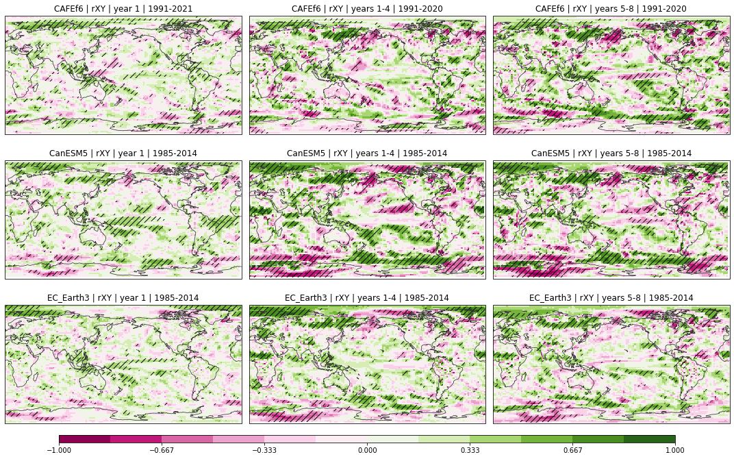
../_images/notebooks_assessment_generic_5_0.png

Anomaly correlation coefficient (Pearson)#

[4]:

_ = plot_metric_maps(["CAFEf6", "CanESM5", "EC_Earth3"], "HadISST", "sst", "rXY")

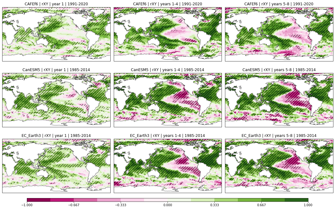
../_images/notebooks_assessment_generic_7_0.png

What are those big patches of negative correlation in the Pacific the 4-year averages?#

These aren’t apparent in Sospedra-Alfonso et al 2021. Are they an artifact of differing “trends” over the short verifcation period? Let’s look at the skill of CanESM5 and EC_Earth3 over a longer (1971-2017) period of time

[5]:

_ = plot_metric_maps(
    ["CanESM5", "EC_Earth3"], "HadISST", "sst", "rXY", verif_period="1971-2017"
)

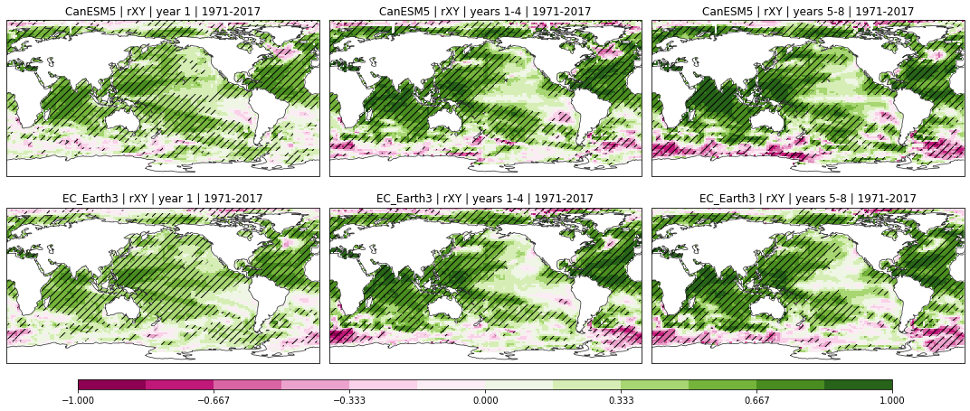
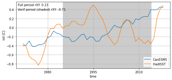
../_images/notebooks_assessment_generic_9_0.png

This looks more like the results in the CanESM5 verification paper. So we need to be pretty careful interpretting the anomaly correlation coefficient over our short verification period. Let’s demonstrate this by looking at the hindcast and observed timeseried at a location in the Pacific:

[6]:

location = dict(lon=225, lat=10)
full_period = slice("1971", "2017")
verif_period = slice("1985", "2014")

hcst = xr.open_zarr(
    "../data/processed/CanESM5.4-year.anom_1985-2014.sst_global.zarr"
).sel(location, method="nearest")
hcst = (
    hcst["sst"]
    .mean("member")
    .sel(lead=59)
    .swap_dims({"init": "time"})
    .sel(time=full_period)
)

obsv = xr.open_zarr(
    "../data/processed/HadISST.4-year.anom_1985-2014.sst_global.zarr"
).sel(location, method="nearest")
obsv = obsv["sst"].sel(time=hcst.time)

acc_full_period = xs.pearson_r(hcst, obsv, dim="time").values.item()

acc_verif_period = xs.pearson_r(
    hcst.sel(time=verif_period), obsv.sel(time=verif_period), dim="time"
).values.item()

[7]:

fig, ax = plt.subplots(figsize=(9, 4))

hcst.plot(label="CanESM5")
obsv.plot(label="HadISST")
ylim = plt.gca().get_ylim()
plt.fill_between(
    [cftime.datetime(1985, 1, 1), cftime.datetime(2014, 1, 1)],
    [ylim[0], ylim[0]],
    [ylim[1], ylim[1]],
    color=[0.8, 0.8, 0.8],
)
plt.gca().set_ylim(ylim)
plt.title("")
plt.legend(loc="lower right")
plt.grid()

plt.text(
    0.01,
    0.98,
    f"Full period rXY: {acc_full_period:.2f}",
    horizontalalignment="left",
    verticalalignment="top",
    transform=ax.transAxes,
)
_ = plt.text(
    0.01,
    0.91,
    f"Verif period (shaded) rXY: {acc_verif_period:.2f}",
    horizontalalignment="left",
    verticalalignment="top",
    transform=ax.transAxes,
)

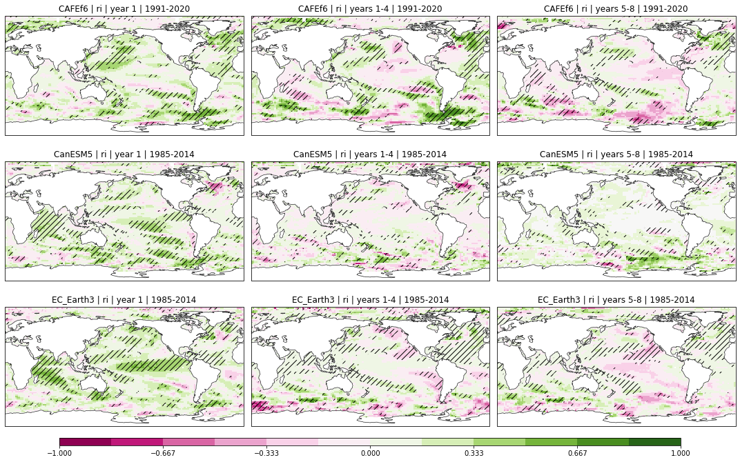
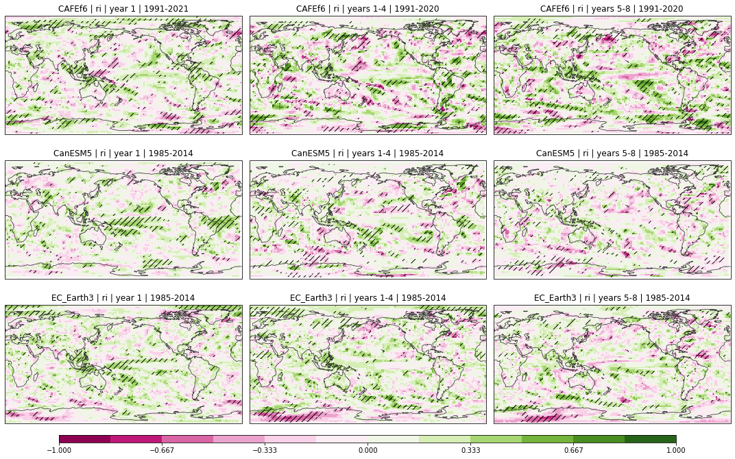
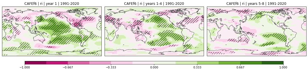
../_images/notebooks_assessment_generic_12_0.png

Initialised component of the anomaly correlation coefficient#

[8]:

_ = plot_metric_maps(["CAFEf6", "CanESM5", "EC_Earth3"], "HadISST", "sst", "ri")

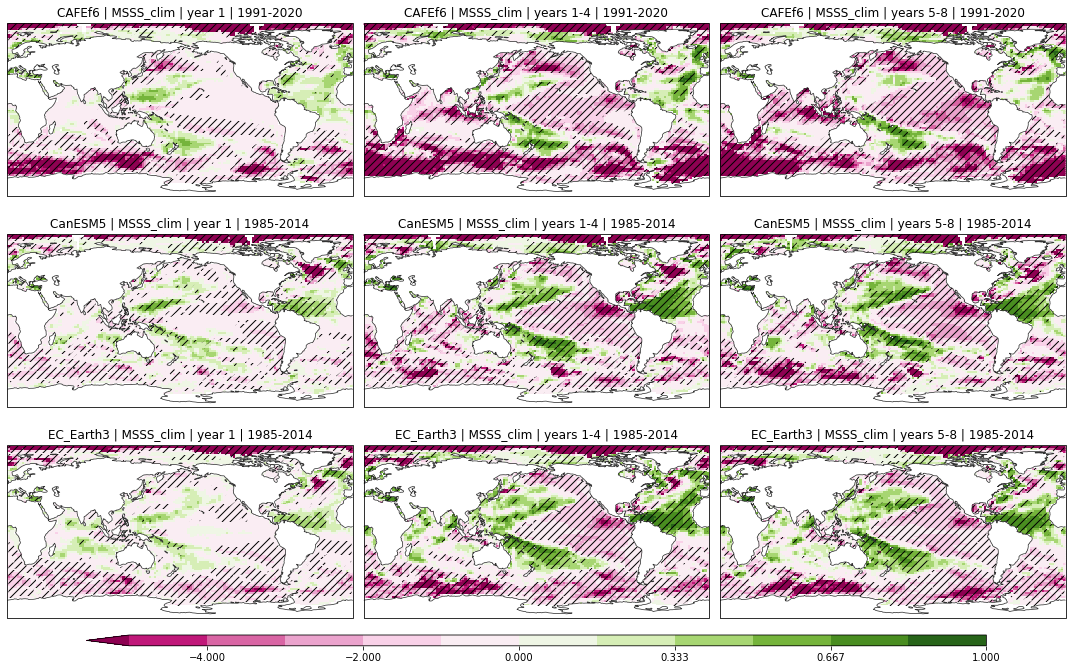
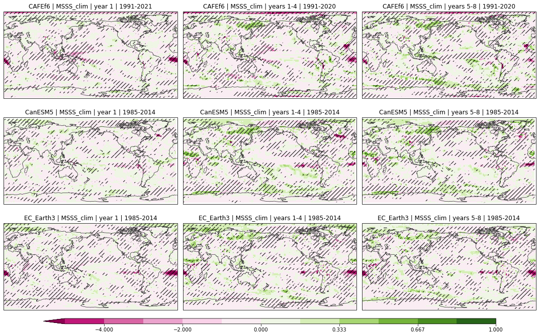
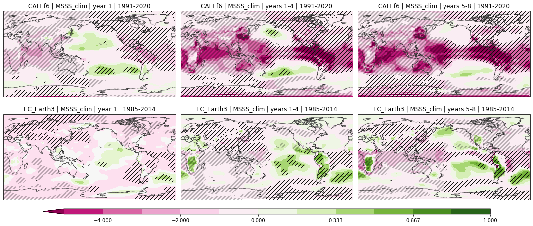
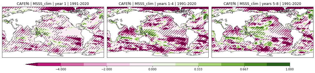
../_images/notebooks_assessment_generic_14_0.png

Mean squared skill score relative to climatology#

[9]:

_ = plot_metric_maps(
    ["CAFEf6", "CanESM5", "EC_Earth3"], "HadISST", "sst", "MSSS_clim", vrange=(-5, 1)
)

../_images/notebooks_assessment_generic_16_0.png

How much does this change for the longer verification period?#

The CanESM5 paper shows large areas in positive skill in the Indian Ocean on the 1-4 year timescales

[10]:

_ = plot_metric_maps(
    ["CanESM5", "EC_Earth3"],
    "HadISST",
    "sst",
    "MSSS_clim",
    verif_period="1971-2017",
    vrange=(-5, 1),
)

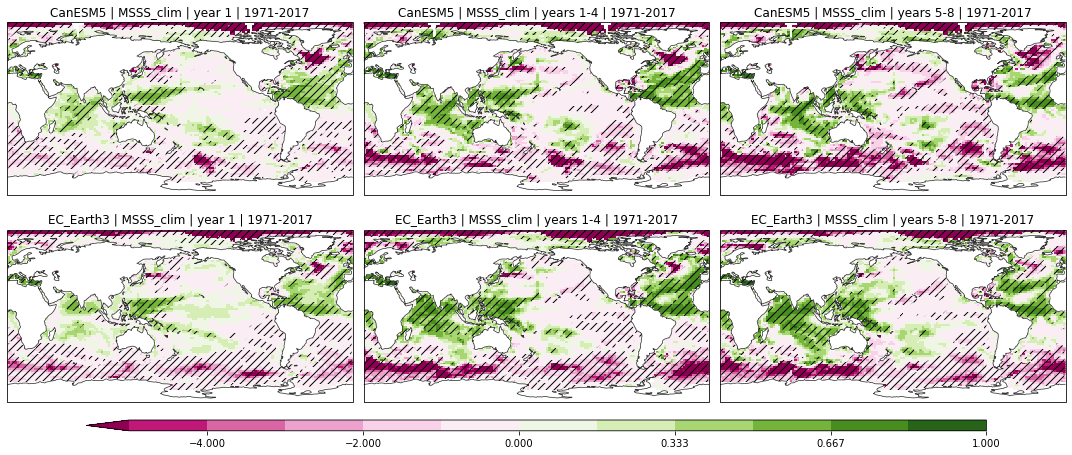
../_images/notebooks_assessment_generic_18_0.png

That looks a little more like the results in the CanESM5 paper

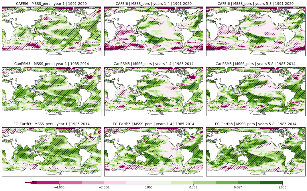
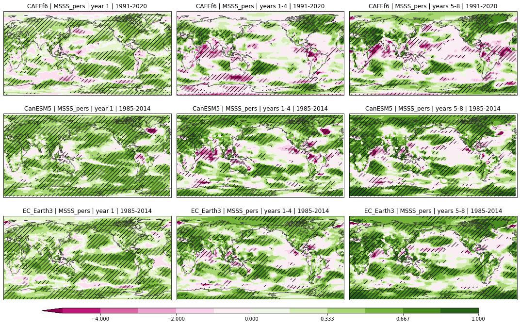
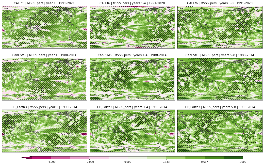
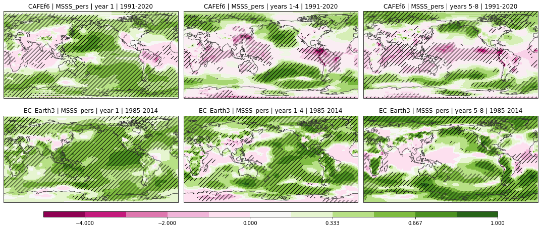
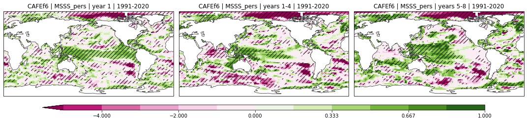
Mean squared skill score relative to persistence#

[11]:

_ = plot_metric_maps(
    ["CAFEf6", "CanESM5", "EC_Earth3"], "HadISST", "sst", "MSSS_pers", vrange=(-5, 1)
)

../_images/notebooks_assessment_generic_21_0.png

How much does this change for the longer verification period?#

The CanESM5 paper shows poorer persistence skill, particularly in the extratropics

[12]:

_ = plot_metric_maps(
    ["CanESM5", "EC_Earth3"],
    "HadISST",
    "sst",
    "MSSS_pers",
    verif_period="1971-2017",
    vrange=(-5, 1),
)

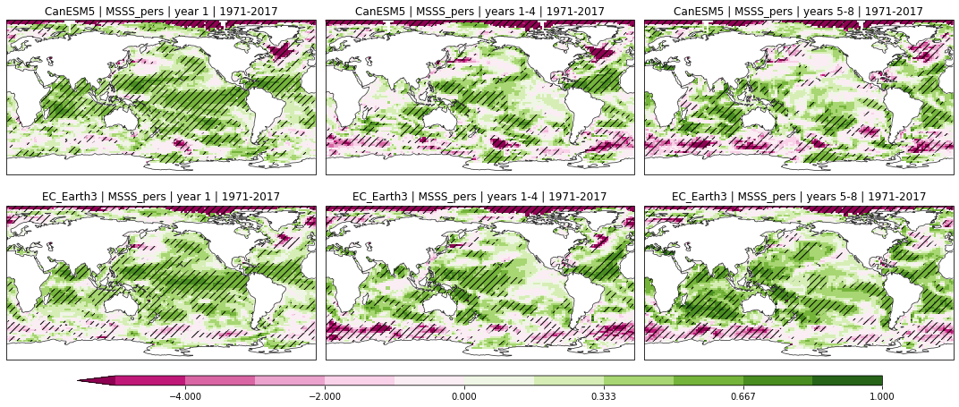
../_images/notebooks_assessment_generic_23_0.png

Still very different that the results in Sospedra-Alfonso et al 2021. It looks as though Sospedra-Alfonso et al 2021 are out by one year in their persistence lag?

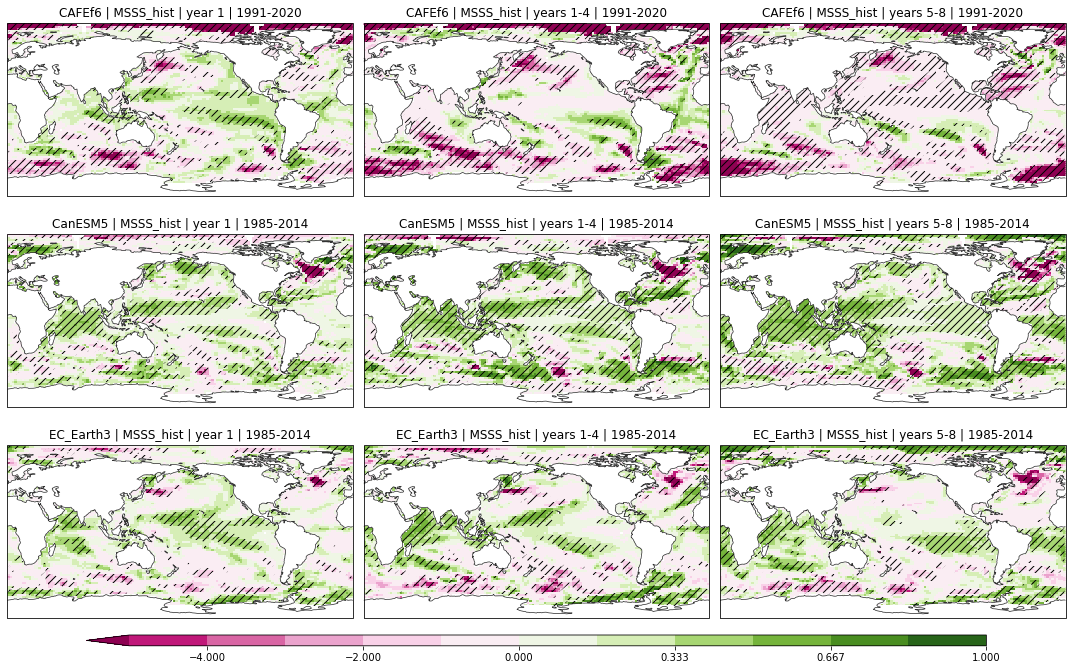
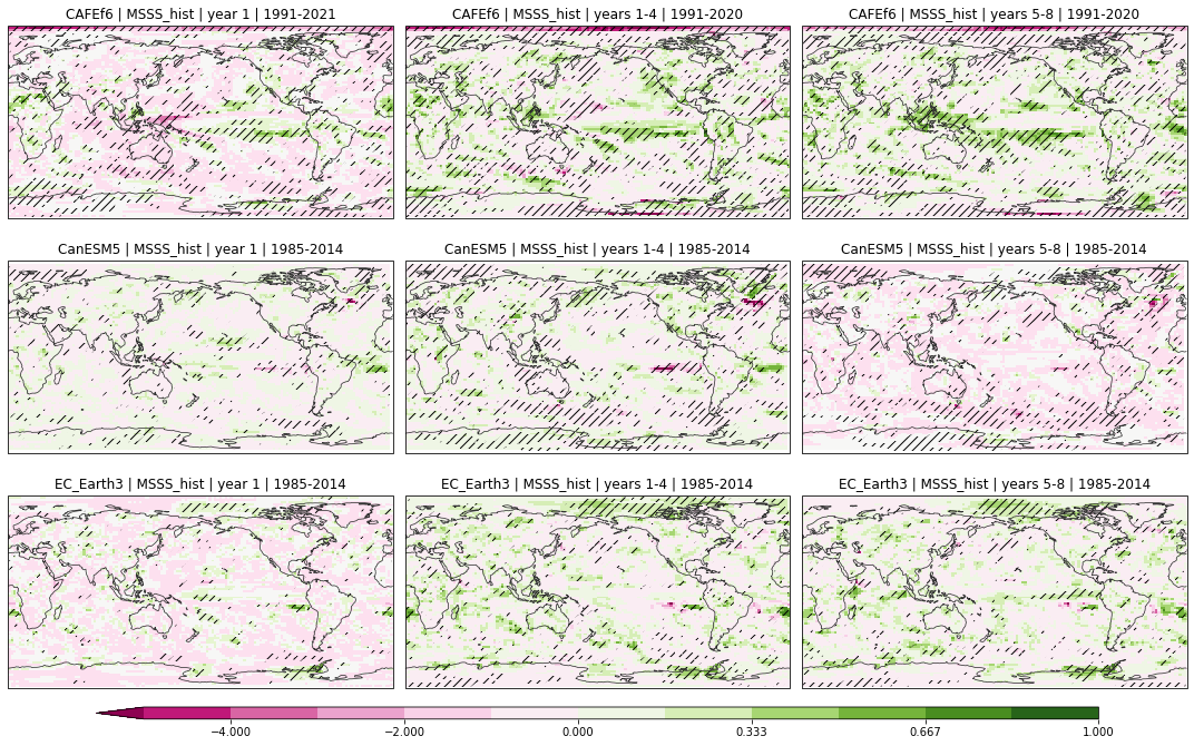
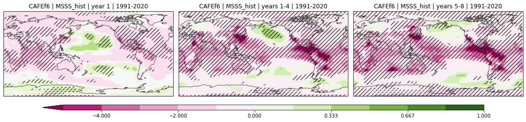
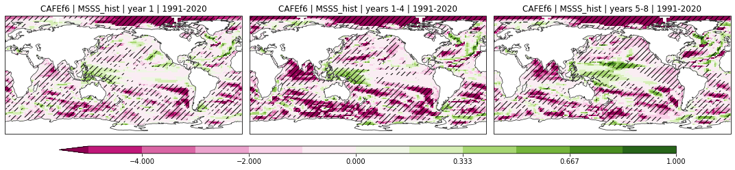
Mean squared skill score relative to historical simulations#

[13]:

_ = plot_metric_maps(
    ["CAFEf6", "CanESM5", "EC_Earth3"], "HadISST", "sst", "MSSS_hist", vrange=(-5, 1)
)

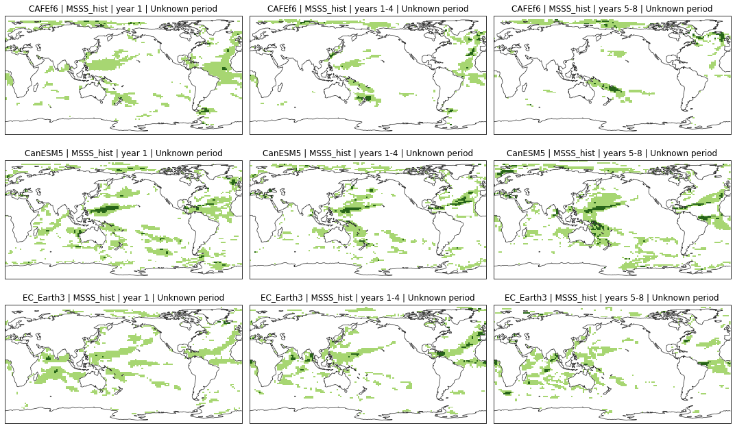
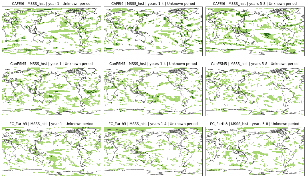
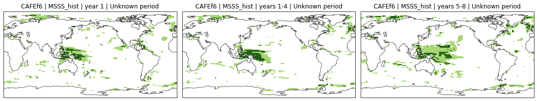
../_images/notebooks_assessment_generic_26_0.png

Where is the MSSS positive relative to climatology, persistence and historical simulations?#

Lighter green indicates both are positive; darker green indicates both are positive and significant

[14]:

_ = plot_metric_maps(
    ["CAFEf6", "CanESM5", "EC_Earth3"],
    "HadISST",
    "sst",
    ["MSSS_clim", "MSSS_pers", "MSSS_hist"],
)

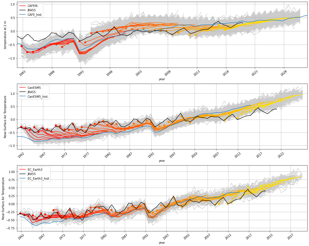
../_images/notebooks_assessment_generic_28_0.png

Near-surface (2m) temperature relative to JRA55#

Global average (60°S - 60°N) hindcast timeseries#

[15]:

plot_hindcasts(
    ["CAFEf6", "CanESM5", "EC_Earth3"],
    ["CAFE_hist", "CanESM5_hist", "EC_Earth3_hist"],
    ["JRA55"],
    "annual",
    "t_ref",
    "global",
)

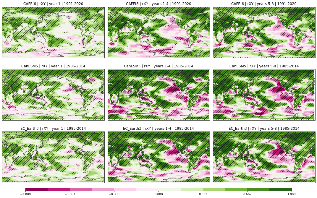
../_images/notebooks_assessment_generic_31_0.png

Anomaly correlation coefficient (Pearson)#

[16]:

_ = plot_metric_maps(["CAFEf6", "CanESM5", "EC_Earth3"], "JRA55", "t_ref", "rXY")

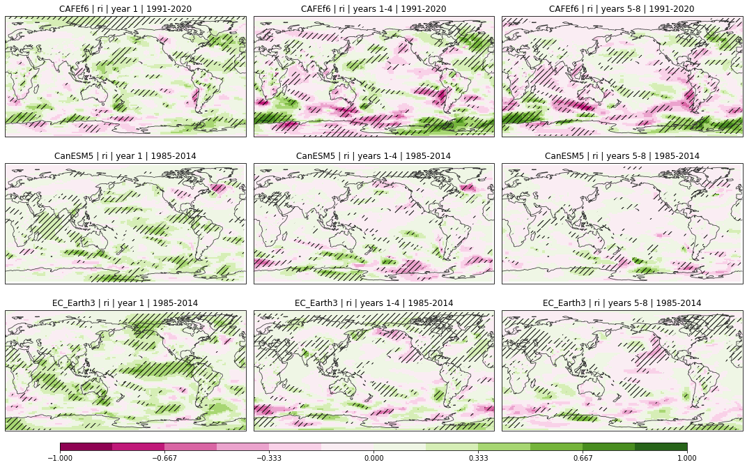
../_images/notebooks_assessment_generic_33_0.png

Initialised component of the anomaly correlation coefficient#

[17]:

_ = plot_metric_maps(["CAFEf6", "CanESM5", "EC_Earth3"], "JRA55", "t_ref", "ri")

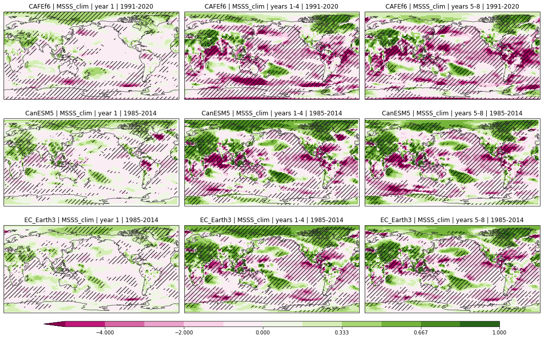
../_images/notebooks_assessment_generic_35_0.png

Mean squared skill score relative to climatology#

[18]:

_ = plot_metric_maps(
    ["CAFEf6", "CanESM5", "EC_Earth3"], "JRA55", "t_ref", "MSSS_clim", vrange=(-5, 1)
)

../_images/notebooks_assessment_generic_37_0.png

Mean squared skill score relative to persistence#

[19]:

_ = plot_metric_maps(
    ["CAFEf6", "CanESM5", "EC_Earth3"], "JRA55", "t_ref", "MSSS_pers", vrange=(-5, 1)
)

../_images/notebooks_assessment_generic_39_0.png

Mean squared skill score relative to historical simulations#

[20]:

_ = plot_metric_maps(
    ["CAFEf6", "CanESM5", "EC_Earth3"], "JRA55", "t_ref", "MSSS_hist", vrange=(-5, 1)
)

../_images/notebooks_assessment_generic_41_0.png

Where is the MSSS positive relative to climatology, persistence and historical simulations?#

Lighter green indicates both are positive; darker green indicates both are positive and significant

[21]:

_ = plot_metric_maps(
    ["CAFEf6", "CanESM5", "EC_Earth3"],
    "JRA55",
    "t_ref",
    ["MSSS_clim", "MSSS_pers", "MSSS_hist"],
)

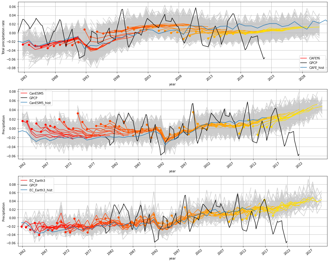
../_images/notebooks_assessment_generic_43_0.png

Precipitation relative to GPCP#

Global average (60°S - 60°N) hindcast timeseries#

[22]:

plot_hindcasts(
    ["CAFEf6", "CanESM5", "EC_Earth3"],
    ["CAFE_hist", "CanESM5_hist", "EC_Earth3_hist"],
    ["GPCP"],
    "annual",
    "precip",
    "global",
)

../_images/notebooks_assessment_generic_46_0.png

Anomaly correlation coefficient (Pearson)#

[23]:

_ = plot_metric_maps(["CAFEf6", "CanESM5", "EC_Earth3"], "GPCP", "precip", "rXY")

../_images/notebooks_assessment_generic_48_0.png

Initialised component of the anomaly correlation coefficient#

[24]:

_ = plot_metric_maps(["CAFEf6", "CanESM5", "EC_Earth3"], "GPCP", "precip", "ri")

../_images/notebooks_assessment_generic_50_0.png

Mean squared skill score relative to climatology#

[25]:

_ = plot_metric_maps(
    ["CAFEf6", "CanESM5", "EC_Earth3"], "GPCP", "precip", "MSSS_clim", vrange=(-5, 1)
)

../_images/notebooks_assessment_generic_52_0.png

Mean squared skill score relative to persistence#

[26]:

_ = plot_metric_maps(
    ["CAFEf6", "CanESM5", "EC_Earth3"], "GPCP", "precip", "MSSS_pers", vrange=(-5, 1)
)

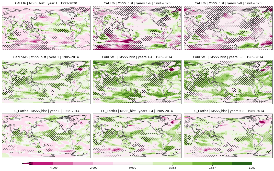
../_images/notebooks_assessment_generic_54_0.png

Mean squared skill score relative to historical simulations#

[27]:

_ = plot_metric_maps(
    ["CAFEf6", "CanESM5", "EC_Earth3"], "GPCP", "precip", "MSSS_hist", vrange=(-5, 1)
)

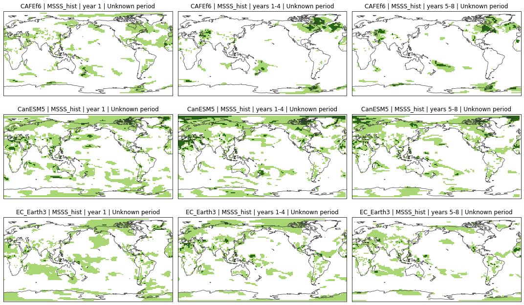
../_images/notebooks_assessment_generic_56_0.png

Where is the MSSS positive relative to climatology, persistence and historical simulations?#

Lighter green indicates both are positive; darker green indicates both are positive and significant

[28]:

_ = plot_metric_maps(
    ["CAFEf6", "CanESM5", "EC_Earth3"],
    "GPCP",
    "precip",
    ["MSSS_clim", "MSSS_pers", "MSSS_hist"],
)

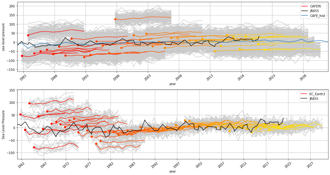
../_images/notebooks_assessment_generic_58_0.png

Sea level pressure relative to JRA55#

Global average (60°S - 60°N) hindcast timeseries#

[29]:

plot_hindcasts(
    ["CAFEf6", "EC_Earth3"],
    ["CAFE_hist"],
    ["JRA55"],
    "annual",
    "slp",
    "global",
)

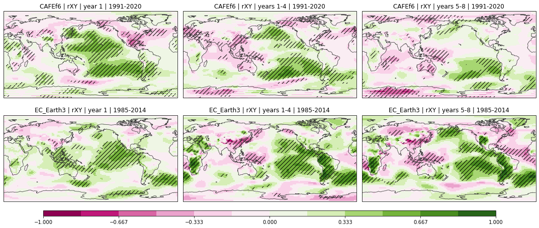
../_images/notebooks_assessment_generic_61_0.png

Anomaly correlation coefficient (Pearson)#

[30]:

_ = plot_metric_maps(["CAFEf6", "EC_Earth3"], "JRA55", "slp", "rXY")

../_images/notebooks_assessment_generic_63_0.png

Initialised component of the anomaly correlation coefficient#

[31]:

_ = plot_metric_maps(["CAFEf6"], "JRA55", "slp", "ri")

../_images/notebooks_assessment_generic_65_0.png

Mean squared skill score relative to climatology#

[32]:

_ = plot_metric_maps(
    ["CAFEf6", "EC_Earth3"], "JRA55", "slp", "MSSS_clim", vrange=(-5, 1)
)

../_images/notebooks_assessment_generic_67_0.png

Mean squared skill score relative to persistence#

[33]:

_ = plot_metric_maps(
    ["CAFEf6", "EC_Earth3"], "JRA55", "slp", "MSSS_pers", vrange=(-5, 1)
)

../_images/notebooks_assessment_generic_69_0.png

Mean squared skill score relative to historical simulations#

[34]:

_ = plot_metric_maps(["CAFEf6"], "JRA55", "slp", "MSSS_hist", vrange=(-5, 1))

../_images/notebooks_assessment_generic_71_0.png

Where is the MSSS positive relative to climatology, persistence and historical simulations?#

Lighter green indicates both are positive; darker green indicates both are positive and significant

[35]:

_ = plot_metric_maps(
    ["CAFEf6"], "JRA55", "slp", ["MSSS_clim", "MSSS_pers", "MSSS_hist"]
)

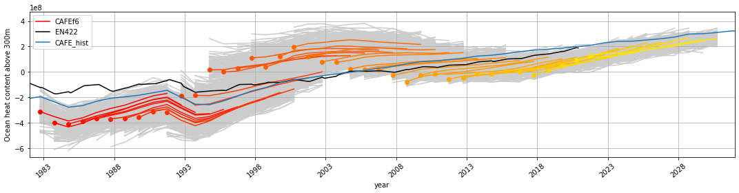
../_images/notebooks_assessment_generic_73_0.png

Upper ocean heat content (upper 300m) relative to EN.4.2.2#

Global average (60°S - 60°N) hindcast timeseries#

[36]:

plot_hindcasts(
    ["CAFEf6"],
    ["CAFE_hist"],
    ["EN422"],
    "annual",
    "ohc300",
    "global",
)

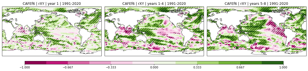
../_images/notebooks_assessment_generic_76_0.png

Anomaly correlation coefficient (Pearson)#

[37]:

_ = plot_metric_maps(["CAFEf6"], "EN422", "ohc300", "rXY")

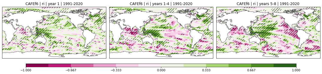
../_images/notebooks_assessment_generic_78_0.png

Initialised component of the anomaly correlation coefficient#

[38]:

_ = plot_metric_maps(["CAFEf6"], "EN422", "ohc300", "ri")

../_images/notebooks_assessment_generic_80_0.png

Mean squared skill score relative to climatology#

[39]:

_ = plot_metric_maps(["CAFEf6"], "EN422", "ohc300", "MSSS_clim", vrange=(-5, 1))

../_images/notebooks_assessment_generic_82_0.png

Mean squared skill score relative to persistence#

[40]:

_ = plot_metric_maps(["CAFEf6"], "EN422", "ohc300", "MSSS_pers", vrange=(-5, 1))

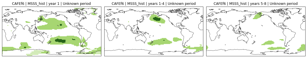
../_images/notebooks_assessment_generic_84_0.png

Mean squared skill score relative to historical simulations#

[41]:

_ = plot_metric_maps(["CAFEf6"], "EN422", "ohc300", "MSSS_hist", vrange=(-5, 1))

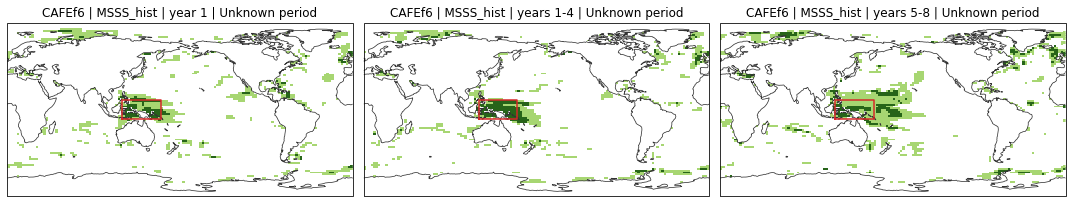
../_images/notebooks_assessment_generic_86_0.png

Where is the MSSS positive relative to climatology, persistence and historical simulations?#

Lighter green indicates both are positive; darker green indicates both are positive and significant

[42]:

ohc300_fig = plot_metric_maps(
    ["CAFEf6"], "EN422", "ohc300", ["MSSS_clim", "MSSS_pers", "MSSS_hist"]
)

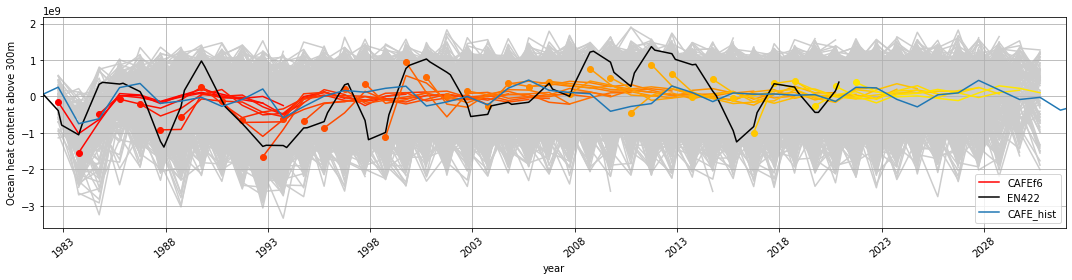
../_images/notebooks_assessment_generic_88_0.png

How do the hindcasts look in the region of positive and significant skill?#

[43]:

box = [120, 160, -10, 10]


def plot_box(ax, box):
    import cartopy.crs as ccrs

    ax.plot(
        [box[0], box[1], box[1], box[0], box[0]],
        [box[2], box[2], box[3], box[3], box[2]],
        "C3",
        transform=ccrs.PlateCarree(),
    )


for ax in ohc300_fig.axes:
    plot_box(ax, box)

ohc300_fig

[43]:

../_images/notebooks_assessment_generic_90_0.png

[44]:

hcst = utils.extract_lon_lat_box(
    xr.open_zarr("../data/processed/CAFEf6.annual.anom_1991-2020.ohc300_global.zarr"),
    box,
    weighted_average=True,
).compute()
hist = utils.extract_lon_lat_box(
    xr.open_zarr(
        "../data/processed/CAFE_hist.annual.anom_1991-2020.ohc300_global.zarr"
    ),
    box,
    weighted_average=True,
).compute()
obsv = utils.extract_lon_lat_box(
    xr.open_zarr("../data/processed/EN422.annual.anom_1991-2020.ohc300_global.zarr"),
    box,
    weighted_average=True,
).compute()

_ = plot.hindcasts({"CAFEf6": hcst}, {"EN422": obsv}, {"CAFE_hist": hist})

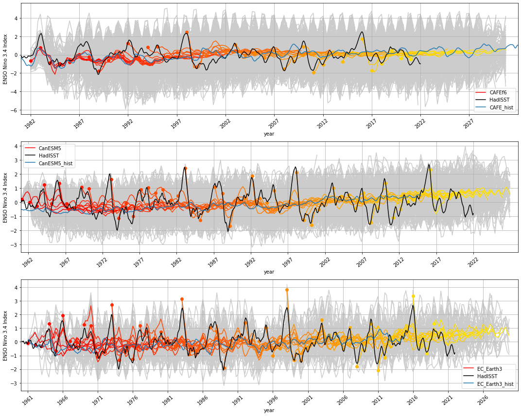
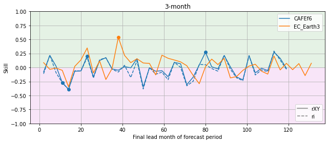
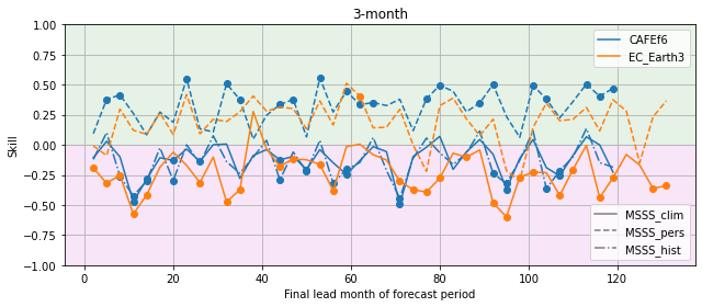
../_images/notebooks_assessment_generic_91_0.png

El-Nino Southern Oscillation relative to HadISST#

(Here, NINO 3.4 is used as an index for the El-Nino Southern Oscillation)

Hindcast timeseries#

[45]:

plot_hindcasts(
    ["CAFEf6", "CanESM5", "EC_Earth3"],
    ["CAFE_hist", "CanESM5_hist", "EC_Earth3_hist"],
    ["HadISST"],
    "3-month",
    "nino34",
)

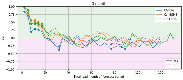
../_images/notebooks_assessment_generic_94_0.png

Anomaly correlation coefficient (Pearson)#

[46]:

_ = plot_metrics(
    ["CAFEf6", "CanESM5", "EC_Earth3"], "HadISST", ["3-month"], "nino34", ["rXY", "ri"]
)

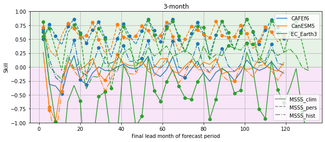
../_images/notebooks_assessment_generic_96_0.png

Mean squared skill score#

[47]:

_ = plot_metrics(
    ["CAFEf6", "CanESM5", "EC_Earth3"],
    "HadISST",
    ["3-month"],
    "nino34",
    ["MSSS_clim", "MSSS_pers", "MSSS_hist"],
)

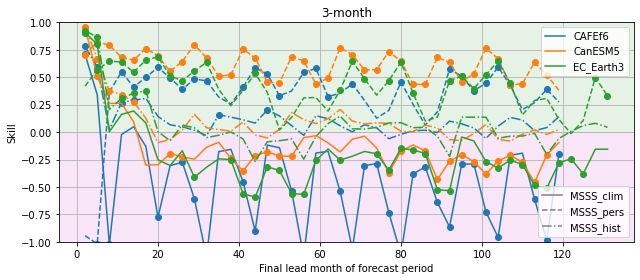
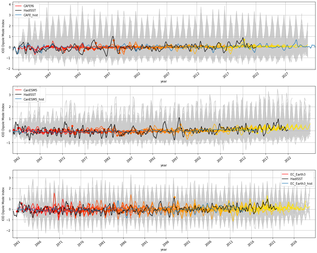
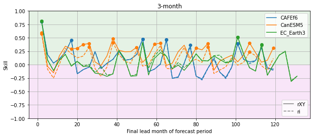
../_images/notebooks_assessment_generic_98_0.png

Indian Ocean Dipole relative to HadISST#

(For the definition of the IOD used here, see Saji and Yamagata 2003)

Hindcast timeseries#

[48]:

plot_hindcasts(
    ["CAFEf6", "CanESM5", "EC_Earth3"],
    ["CAFE_hist", "CanESM5_hist", "EC_Earth3_hist"],
    ["HadISST"],
    "3-month",
    "dmi",
)

../_images/notebooks_assessment_generic_101_0.png

Anomaly correlation coefficient (Pearson)#

[49]:

_ = plot_metrics(
    ["CAFEf6", "CanESM5", "EC_Earth3"], "HadISST", ["3-month"], "dmi", ["rXY", "ri"]
)

../_images/notebooks_assessment_generic_103_0.png

Mean squared skill score#

[50]:

_ = plot_metrics(
    ["CAFEf6", "CanESM5", "EC_Earth3"],
    "HadISST",
    ["3-month"],
    "dmi",
    ["MSSS_clim", "MSSS_pers", "MSSS_hist"],
)

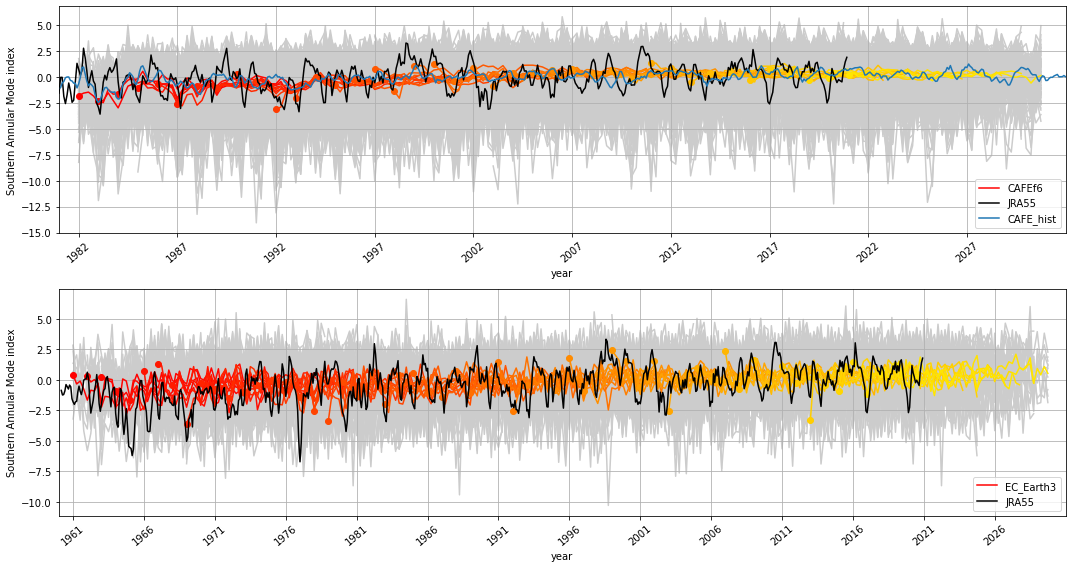
../_images/notebooks_assessment_generic_105_0.png

Southern Annual Mode relative to JRA55#

(For the definition of the SAM used here, see Gong and Wang 1999)

Hindcast timeseries#

[51]:

plot_hindcasts(
    ["CAFEf6", "EC_Earth3"],
    ["CAFE_hist"],
    ["JRA55"],
    "3-month",
    "sam",
)

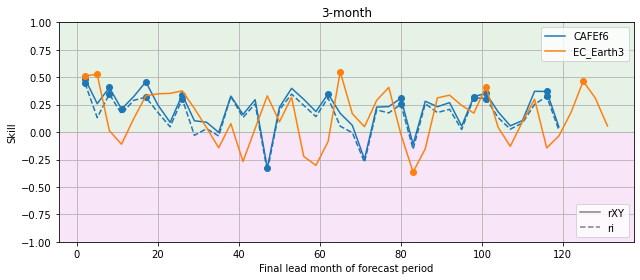
../_images/notebooks_assessment_generic_108_0.png

Anomaly correlation coefficient (Pearson)#

[52]:

_ = plot_metrics(["CAFEf6", "EC_Earth3"], "JRA55", ["3-month"], "sam", ["rXY", "ri"])

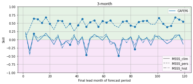
../_images/notebooks_assessment_generic_110_0.png

Mean squared skill score#

[53]:

_ = plot_metrics(
    ["CAFEf6"], "JRA55", ["3-month"], "sam", ["MSSS_clim", "MSSS_pers", "MSSS_hist"]
)

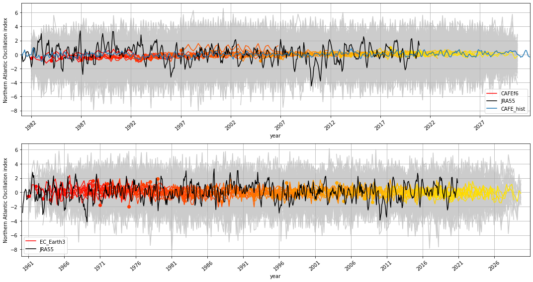
../_images/notebooks_assessment_generic_112_0.png

North Atlantic Oscillation Index relative to JRA55#

(For the definition of the NAO used here, see Jianping and Wang)

Hindcast timeseries#

[54]:

plot_hindcasts(
    ["CAFEf6", "EC_Earth3"],
    ["CAFE_hist"],
    ["JRA55"],
    "3-month",
    "nao",
)

../_images/notebooks_assessment_generic_115_0.png

Anomaly correlation coefficient (Pearson)#

[55]:

_ = plot_metrics(["CAFEf6", "EC_Earth3"], "JRA55", ["3-month"], "nao", ["rXY", "ri"])

../_images/notebooks_assessment_generic_117_0.png

Mean squared skill score#

[56]:

_ = plot_metrics(
    ["CAFEf6", "EC_Earth3"],
    "JRA55",
    ["3-month"],
    "nao",
    ["MSSS_clim", "MSSS_pers", "MSSS_hist"],
)

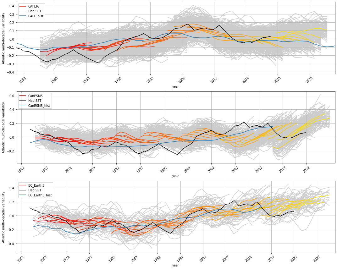
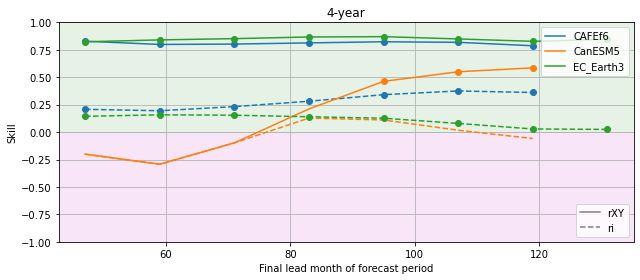
../_images/notebooks_assessment_generic_119_0.png

Atlantic multi-decadal variability relative to HadISST#

(For the definition of the AMV used here, see Trenberth and Shea 2006)

Hindcast timeseries#

[57]:

plot_hindcasts(
    ["CAFEf6", "CanESM5", "EC_Earth3"],
    ["CAFE_hist", "CanESM5_hist", "EC_Earth3_hist"],
    ["HadISST"],
    "4-year",
    "amv",
)

../_images/notebooks_assessment_generic_122_0.png

Anomaly correlation coefficient (Pearson)#

[58]:

_ = plot_metrics(
    ["CAFEf6", "CanESM5", "EC_Earth3"], "HadISST", ["4-year"], "amv", ["rXY", "ri"]
)

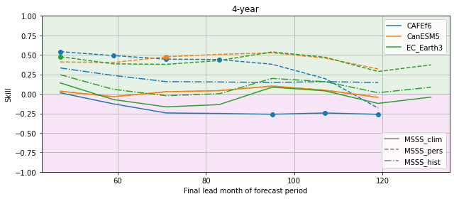
../_images/notebooks_assessment_generic_124_0.png

Mean squared skill score#

[59]:

_ = plot_metrics(
    ["CAFEf6", "CanESM5", "EC_Earth3"],
    "HadISST",
    ["4-year"],
    "amv",
    ["MSSS_clim", "MSSS_pers", "MSSS_hist"],
)

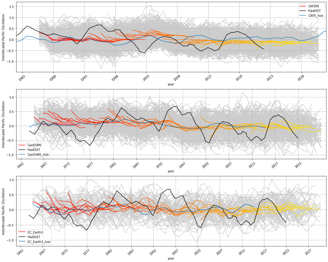
../_images/notebooks_assessment_generic_126_0.png

Inter-decadal Pacific oscillation relative to HadISST#

(For the definition of the IPO used here, see Henley et al 2015)

Hindcast timeseries#

[60]:

plot_hindcasts(
    ["CAFEf6", "CanESM5", "EC_Earth3"],
    ["CAFE_hist", "CanESM5_hist", "EC_Earth3_hist"],
    ["HadISST"],
    "4-year",
    "ipo",
)

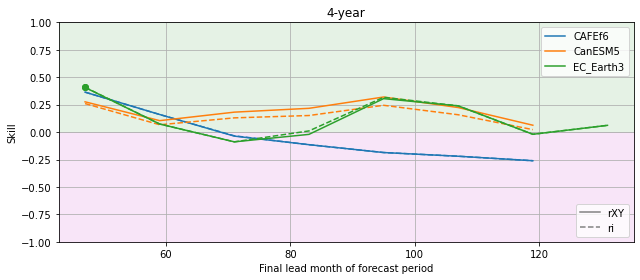
../_images/notebooks_assessment_generic_129_0.png

Anomaly correlation coefficient (Pearson)#

[61]:

_ = plot_metrics(
    ["CAFEf6", "CanESM5", "EC_Earth3"], "HadISST", ["4-year"], "ipo", ["rXY", "ri"]
)

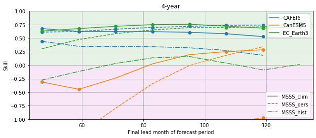
../_images/notebooks_assessment_generic_131_0.png

Mean squared skill score#

[62]:

_ = plot_metrics(
    ["CAFEf6", "CanESM5", "EC_Earth3"],
    "HadISST",
    ["4-year"],
    "ipo",
    ["MSSS_clim", "MSSS_pers", "MSSS_hist"],
)

../_images/notebooks_assessment_generic_133_0.png